Neutron transport and capture spectrum

Historically, the simulation of low-energetic neutron transport and capture has faced several challenges and limitations. In the current Geant4 versions, this is commonly handled by the Neutron high-precision (NeutronHP/ParticleHP) model. There, neutron interactions below ~20 MeV are modelled using the Geant4 Neutron Data Library (G4NDL), which is derived from evaluated nuclear data libraries such as ENDF/B, JEFF or JENDL. These libraries contain experimentally measured and theoretically evaluated cross sections, enabling a detailed and isotope-resolved description of neutron transport.

The user of Geant4 has the option to install and use many different evaluated libraries as explained here. This validation suite focuses on the data libraries that come distributed with the Geant4 installation of remage. As of G4NDL4.7.1 these are mostly based on JEFF-3.3.

Note

The installation of new neutron data libraries should work the same way as for basic Geant4. Copy the libraries in the corresponding folders (which should either be under "/opt/geant4/share/Geant4/data" or under $CONDA_PREFIX/share/Geant4/data, depending on the type of installation) and point the G4NEUTRONHPDATA variable to them.

remage allows for the specification of hadronic physics with the macro command /RMG/Processes/HadronicPhysics as explained in the Hadronic Physics Options section. This validation will focus on the Shielding option for hadronic physics. Additionally, remage allows for a modification of the neutron capture process according to this section, which will also be validated.

The materials tested in these validations are chosen based on their relevance for particle physics experiments, such as LEGEND-1000.

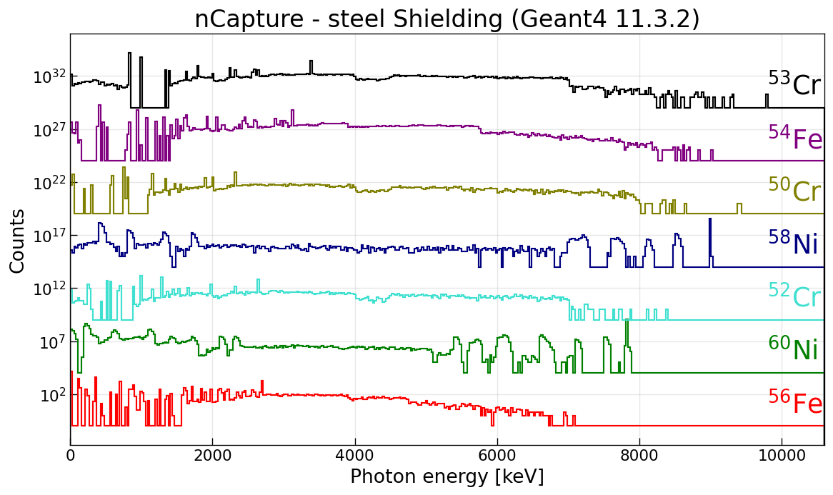
Steel captures

This is a simple world filled with the nist material "G4_STAINLESS-STEEL". Here, the gamma spectrum after the nCapture is examined. The only active process for neutrons is nCapture and neutrons are sampled at 10 keV. The goal is to validate or compare the spectrum against other models, which are missing for now. All isotopes are illustrated in the same histogram. For this, each isotope is shifted up by a constant offset.

Todo

Add spectra of other models for comparison

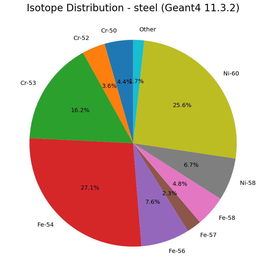
Additionally, a pie-chart showing the distribution of the neutron captures results as a by-product and can be shown. This can be used to validate the nCapture cross-sections of steel at 10 keV. The material G4_STAINLESS-STEEL is made out of 74% iron, 18% chromium and 8% nickel. Despite iron consisting to 91.8% out of Fe-56, we would not necessarily expect Fe-56 to have the main contribution at 10 keV. This is because 10 keV is right in the resonance-area and the cross section heavily depends on the actual database you are using. The same applies to the other elements.

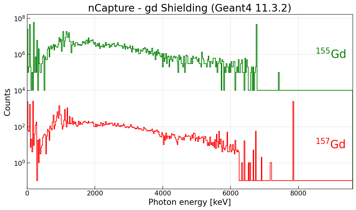
Geant4 nCapture vs RMGnCapture

In this simple world filled with "G4_Gd", the only active process again is either nCapture or RMGnCapture. The purpose of RMGnCapture is documented here. The neutrons are sampled at 0.1 eV. The pie-charts show the capture distribution on the gadolinium isotopes. They are expected to show the same thing in both cases, as the RMGnCapture process should only impact the gamma cascade and not the capture cross-section.

Distribution using the Geant4 `nCapture`.

Distribution using the custom `RMGnCapture`.

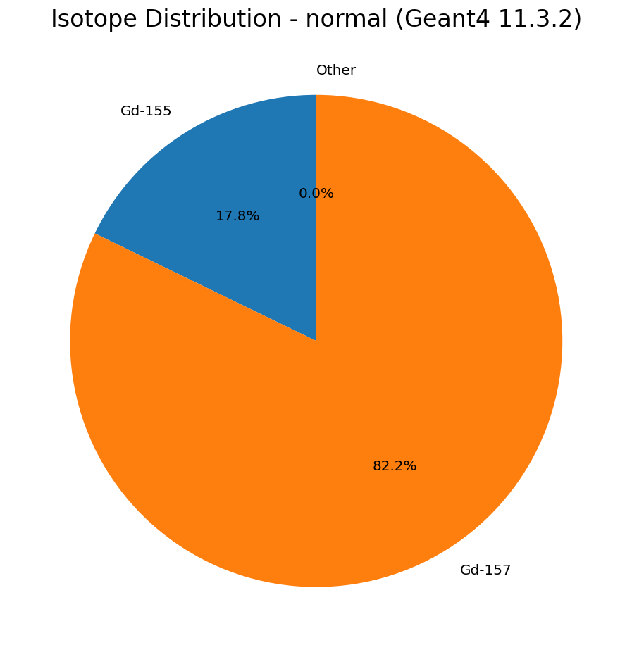
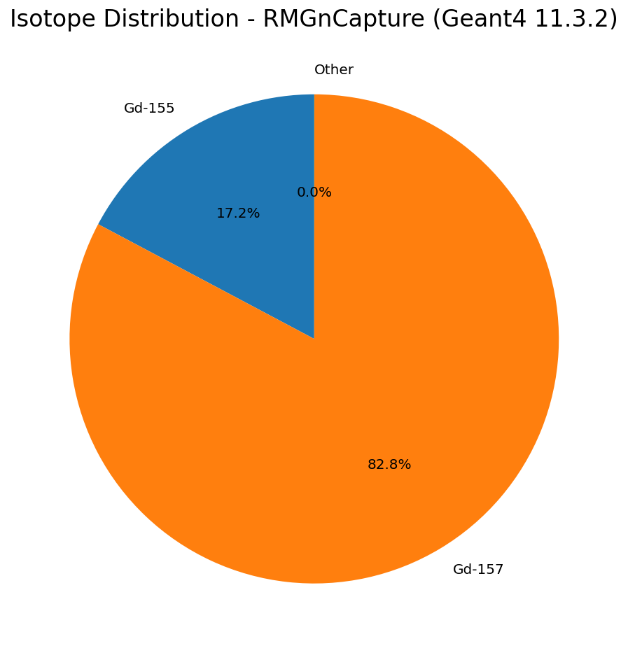
If both plots do not show the same thing (within an expected ~1% relative deviation based on 10 000 simulated neutrons) there is an issue.

We can also take a look at the de-excitation gamma spectrum:

Relative cross-section of gadolinium

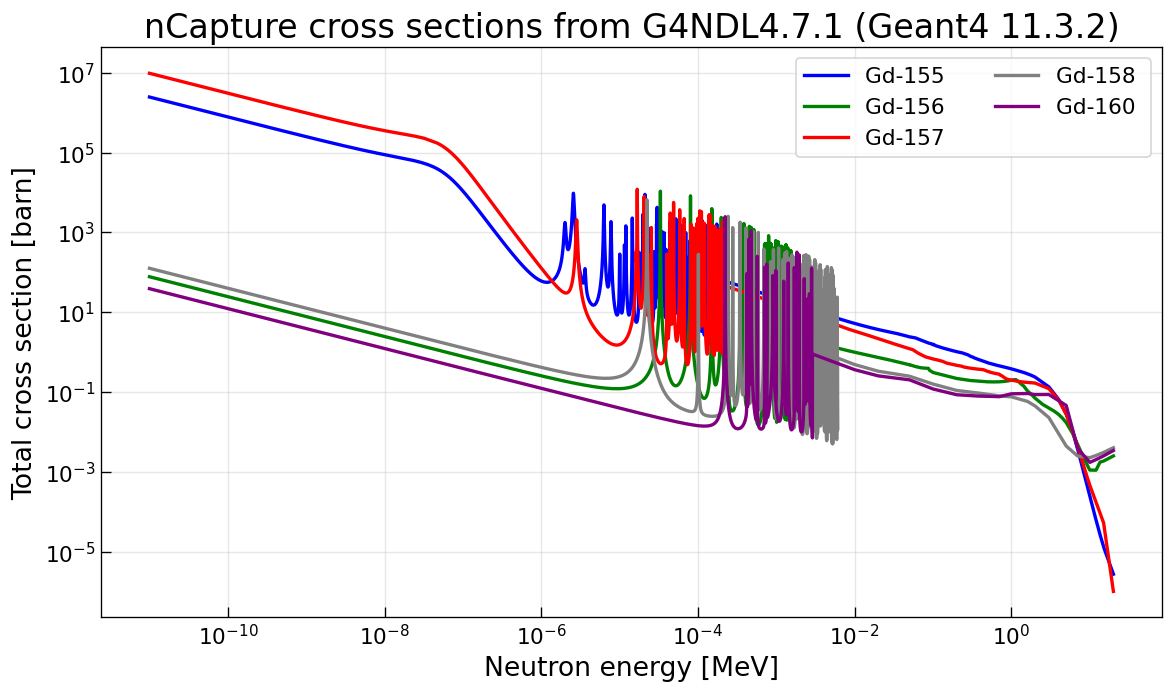
This setup re-creates the relative cross-section of nCapture on gadolinium and validates it against the literature. As before, the world is a simple volume consisting of "G4_Gd" and the only active process for neutrons is nCapture. Neutrons are sampled with a log-uniform distribution from 0.01 eV to 1 MeV. First we take a look at the latest G4NDL data that is stored for Geant4, to see if it exists and is reasonable. This means the data in the next figure is dynamically extracted out of the data folder part of the Geant4 installation. There should be data displayed for Gd-155, Gd-156, Gd-157, Gd-158 and Gd-160.

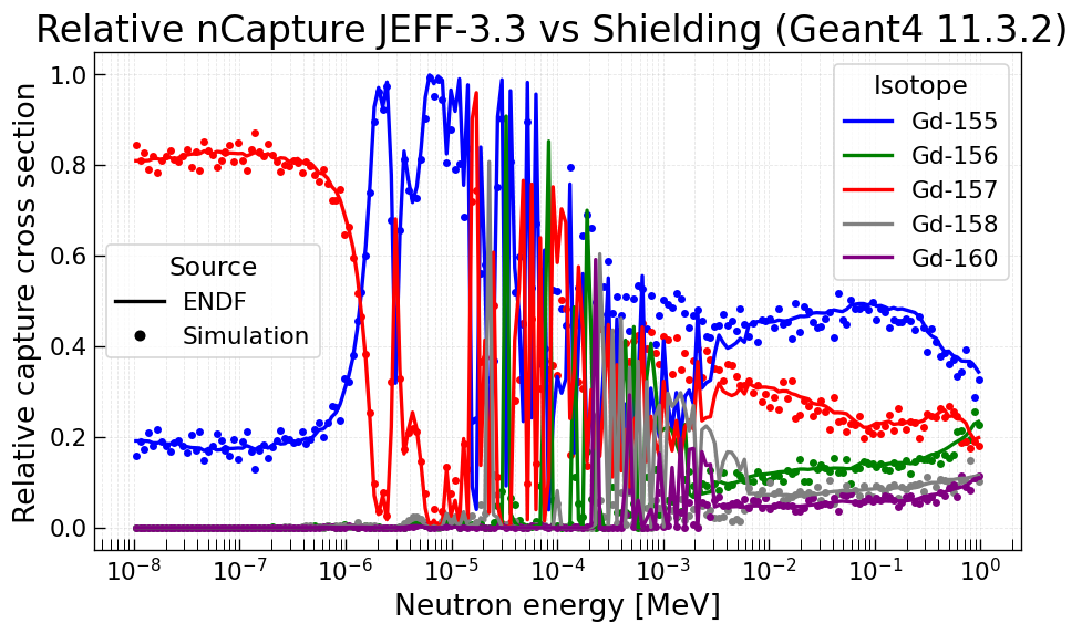
Next, the relative nCapture cross-section for gadolinium is reconstructed and compared to the nCapture cross-section according to JEFF-3.3. Each isotope was weighted by the natural abundance in gadolinium and the relative fraction of the total nCapture cross-section was derived. Additionally, the data was re-binned to fit to the binning of the simulation. The relative cross-section from the simulation was re-constructed by counting the number of captures on each isotope at given energy.

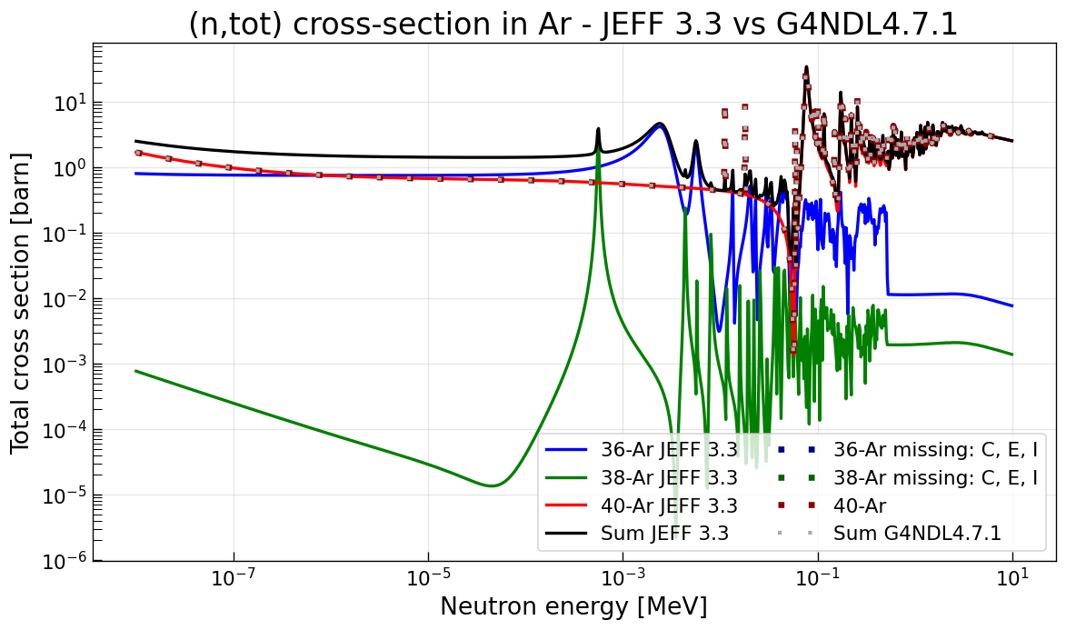
Argon transport

Here, we validate neutron transport in argon. First, the total cross-section for neutrons with the different argon isotopes is compared. For this, Geant4 typically uses G4NDL data. In the following plots, the latest G4NDL data is directly (dynamically) extracted out of the data folder part of the Geant4 installation. The solid lines shows the static JEFF-3.3 data (on which at least G4NDL4.7 is based on), while the corresponding dots (squares) show the latest G4NDL data. Both data has been scaled with the natural isotope fraction. It can be possible, that G4NDL data is missing for certain isotopes. This is indicated by the label stating “missing: …”. The letters stand for : “C” means the “Capture” data is missing, “E” means the “elastic scattering” data is missing and “I” means the “inelastic scattering” data is missing.

Note

In G4NDL4.7.1 the cross-sections for Ar36 and Ar38 were removed according to the patch notes. This means unless they are re-added in future versions a disagreement with JEFF is expected and should be monitored carefully.

To not only verify the data files, but also that they get applied correctly and the simulation works, the total cross-section for neutrons in liquid Argon is reconstructed from an idealized simulation. In this idealized simulation an orb of 2 km radius is used. There are three worlds and three simulations, one for each argon isotope. The density (and temperature) of the argon is that of liquid argon. Every process is active and the Neutrons are sampled from a log-uniform distribution from 0.01 eV to 10 MeV. To calculate the total cross-sections, first the step length between two steps is derived, using the position of each step. The mean of this value is taken as mean free path and used to derive the total cross-section. The energy is given by the velocity of the particle at pre-step. Due to the 2 km radius of the orb, geometric boundaries should not be relevant. Additionally, a distance to surface check only counts those events, that end up at least 10 m away from any boundary. Still, the results look like there might be a bias from the simulation. This could be caused by non-physical simulation processes limiting the step length.

Todo

Investigate the effect of non-physical simulation processes on this cross-section reconstruction. Possibly by setting up a thin target neutron beam experiment.

The plot shows the total weighted cross-section for natural argon according to JEFF-3.3, G4NDL and using this reconstruction method.

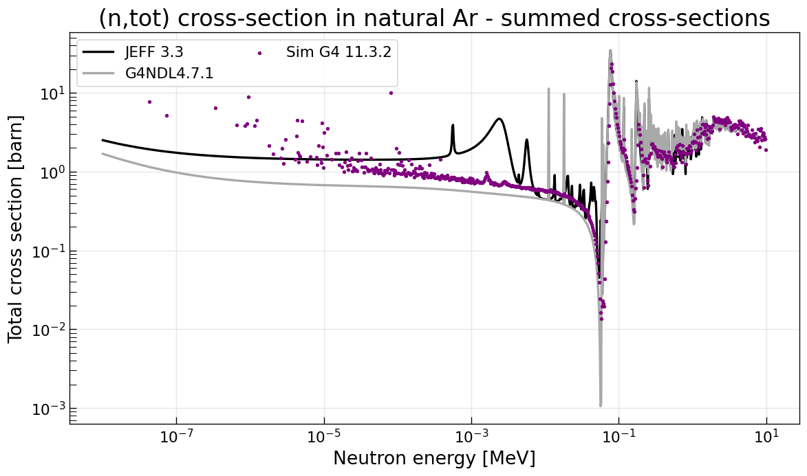
Because some isotopes might be missing in G4NDL, it can be possible that the simulation does not reproduce the G4NDL prediction. It might therefore be useful to investigate the cross-sections for the individual isotopes again:

argon-36 total cross-section.

argon-38 total cross-section.

argon-40 total cross-section.

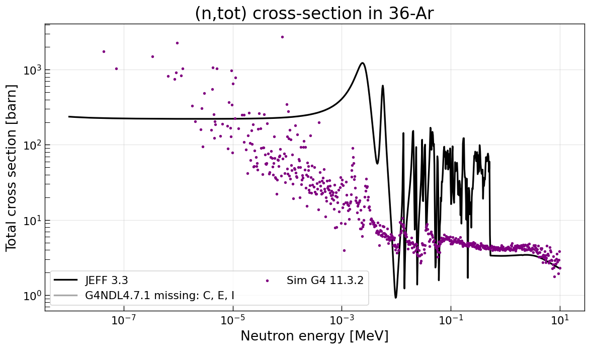
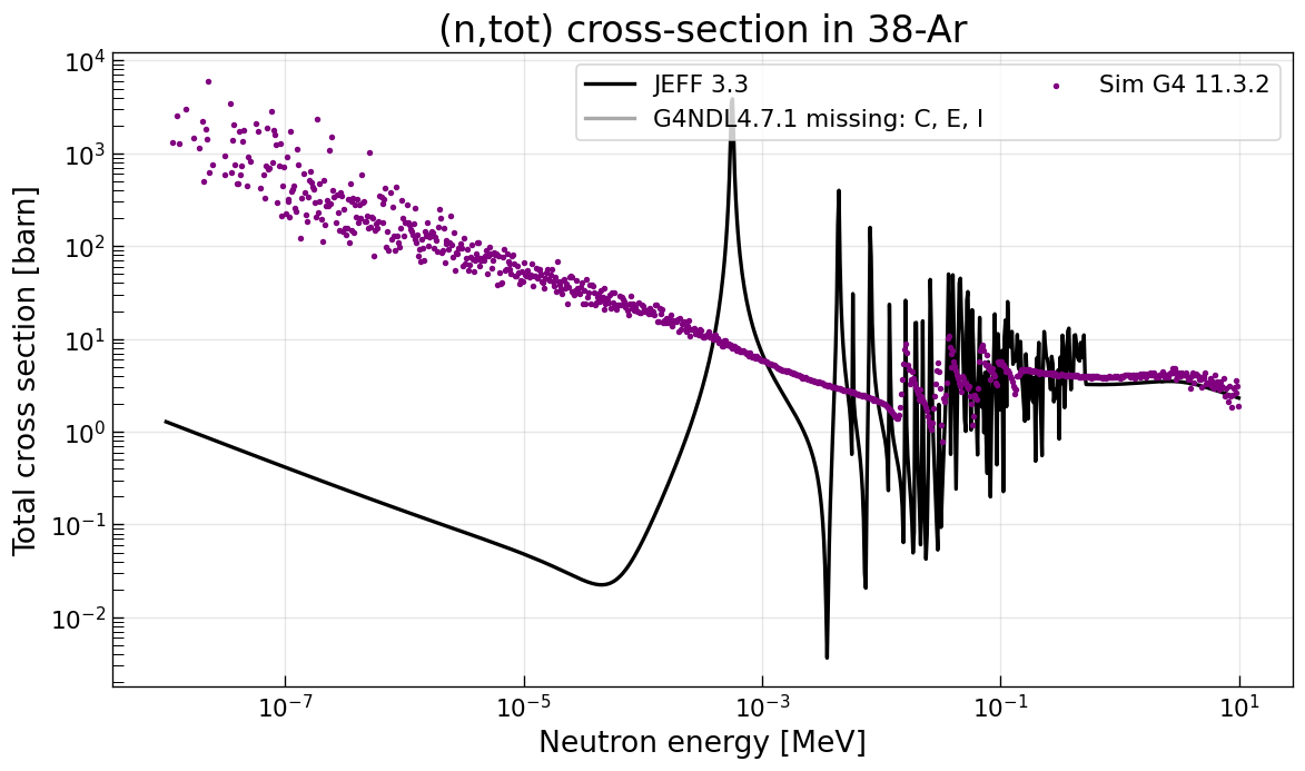
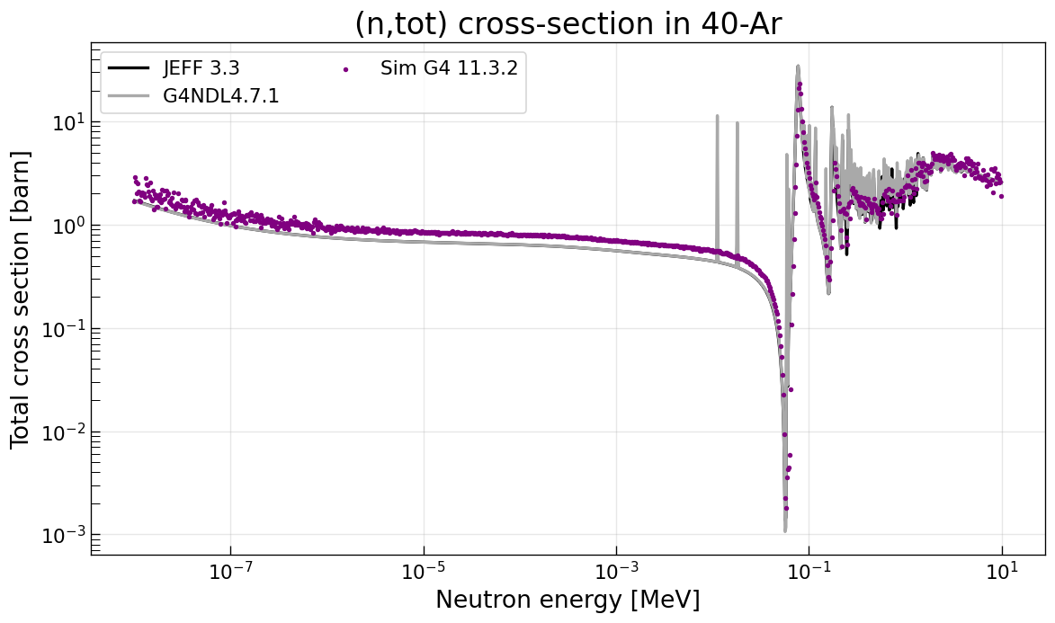
The total cross-sections of the three stable argon isotopes.

For cases where the G4NDL cross-section is missing, Geant4 might fall back to use the cross-section of similar isotopes instead.

Complex geometry

Last, we try to show some parameters simulating a more complex world, similar to many particle physics experiments. Neutrons are sampled at 5 keV but every process is active. Neutrons are simulated in a steel container filled with liquid argon. The steel container itself is located within a water volume and inside of the argon there is also a neutron moderator, which consists of hydrogen and is loaded with gadolinium. The goal of the geometry is to enable not only neutron capture on different isotopes, but also to have the neutron transport be a crucial component regarding capture distribution. The main elements on which can be captured in this geometry are therefore H, Ar, Cr, Fe, Ni, Gd.

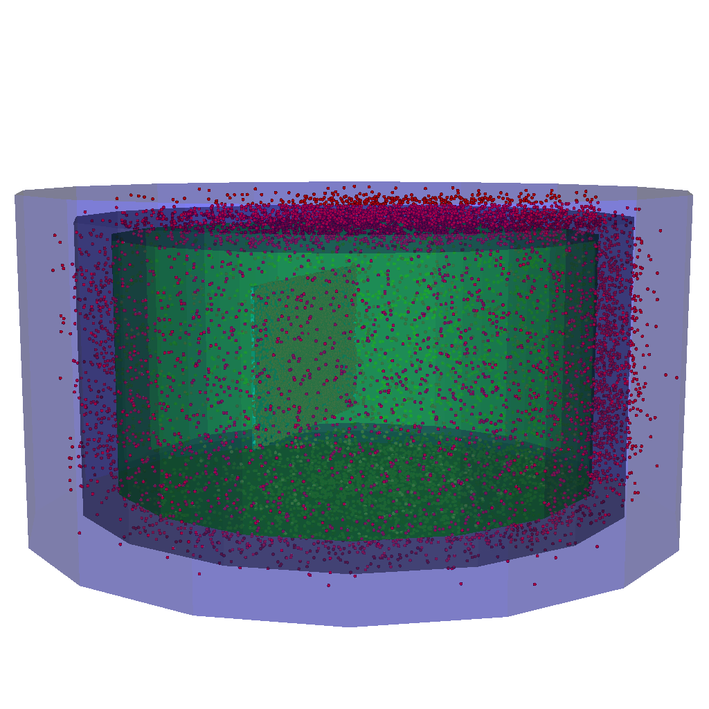
An image of this setup. The moderator in cyan, argon in green, steel in a darker gray and water in blue. The dots represent the positions of neutron captures.

First, the pie-chart showing where the captures took place is shown:

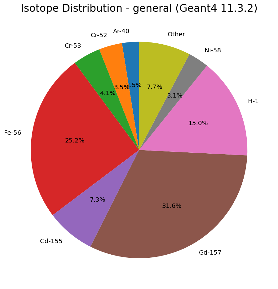
While this pie-chart can not be compared to literature values, as it also heavily depends on the neutron transport, it can be compared between remage versions.

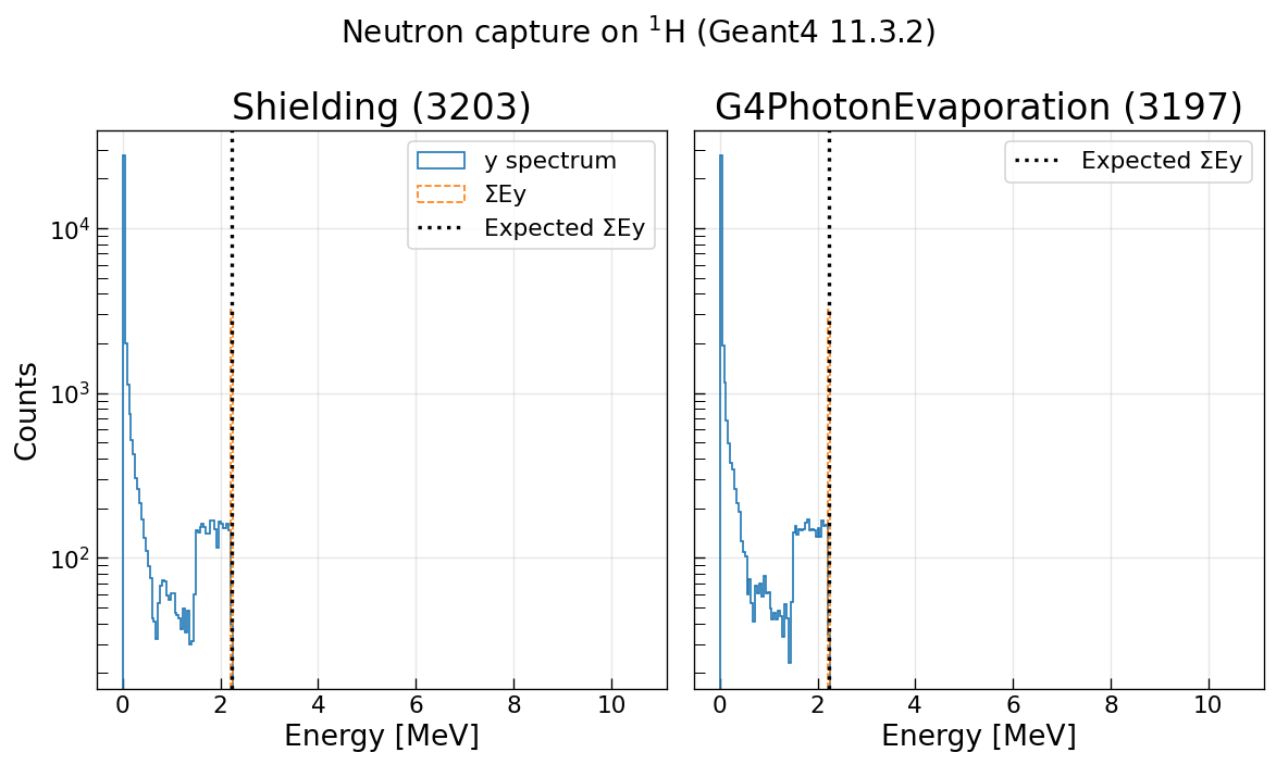
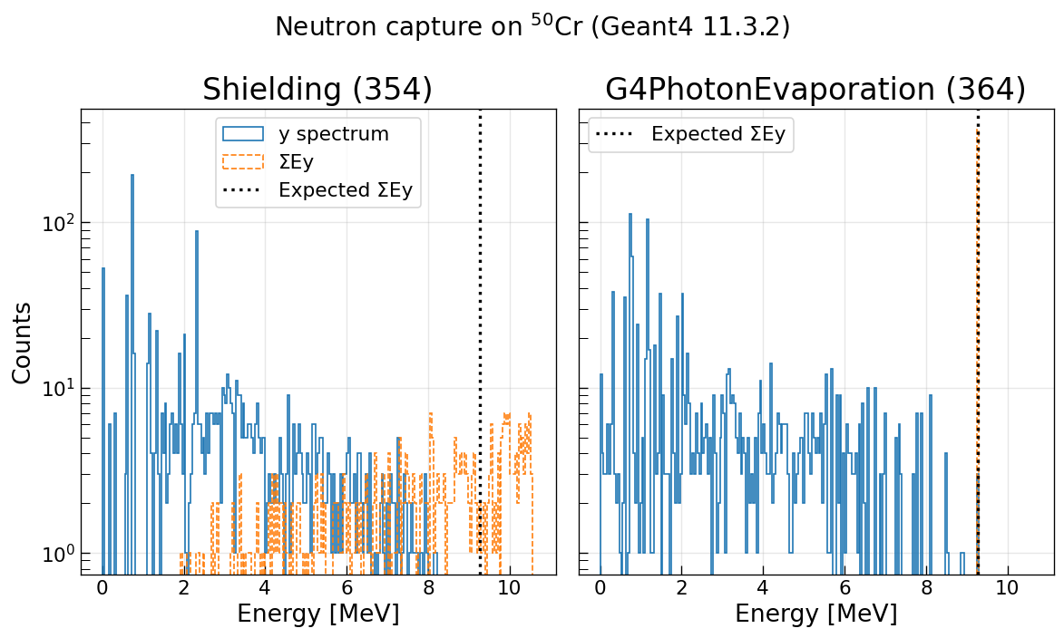
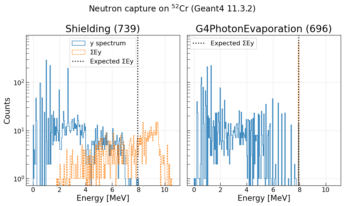
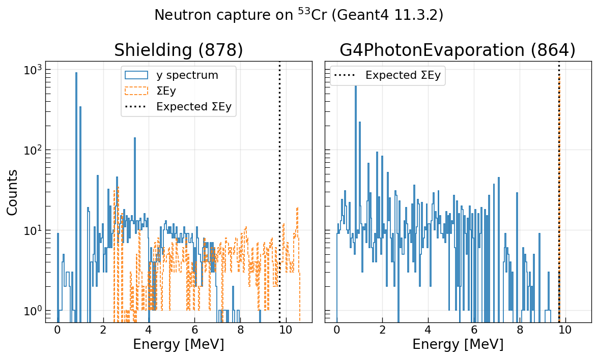
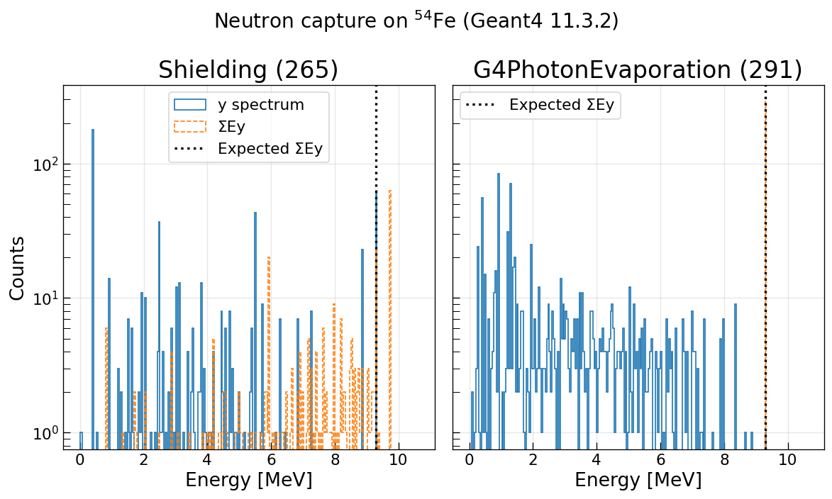
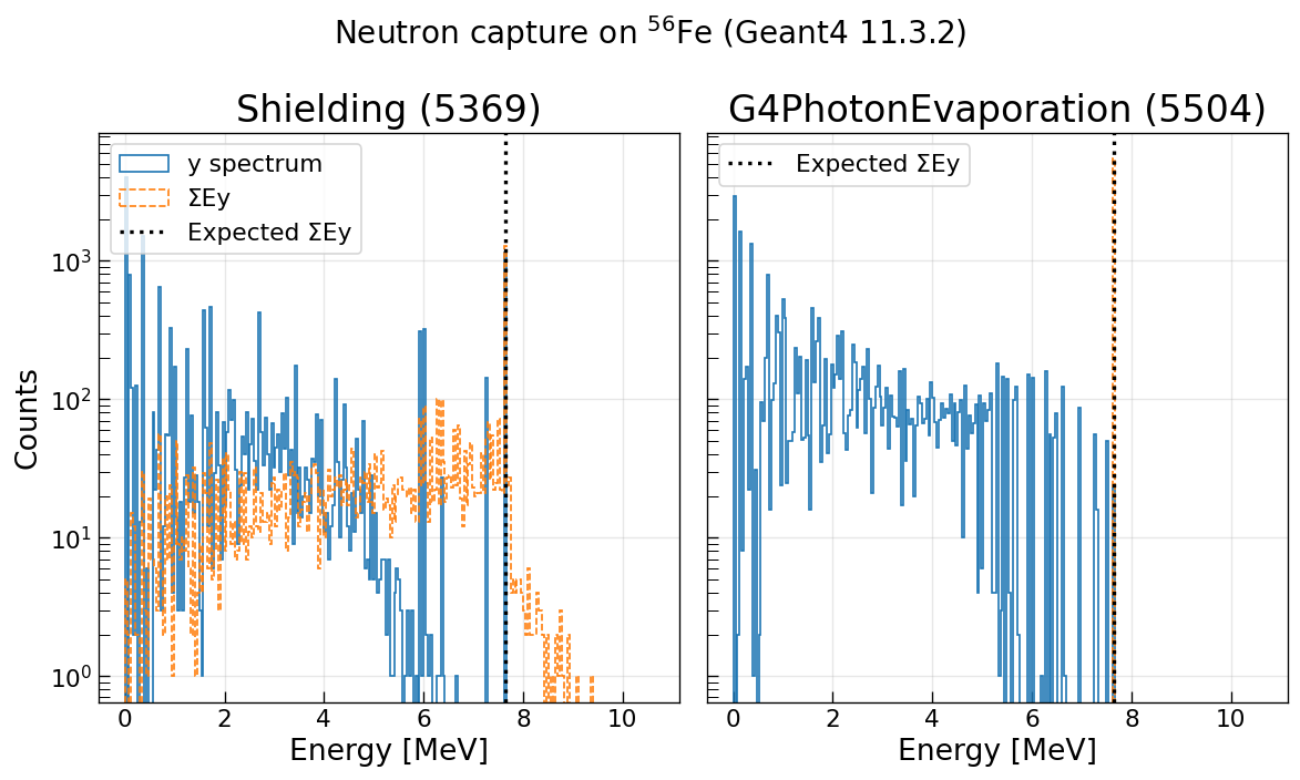
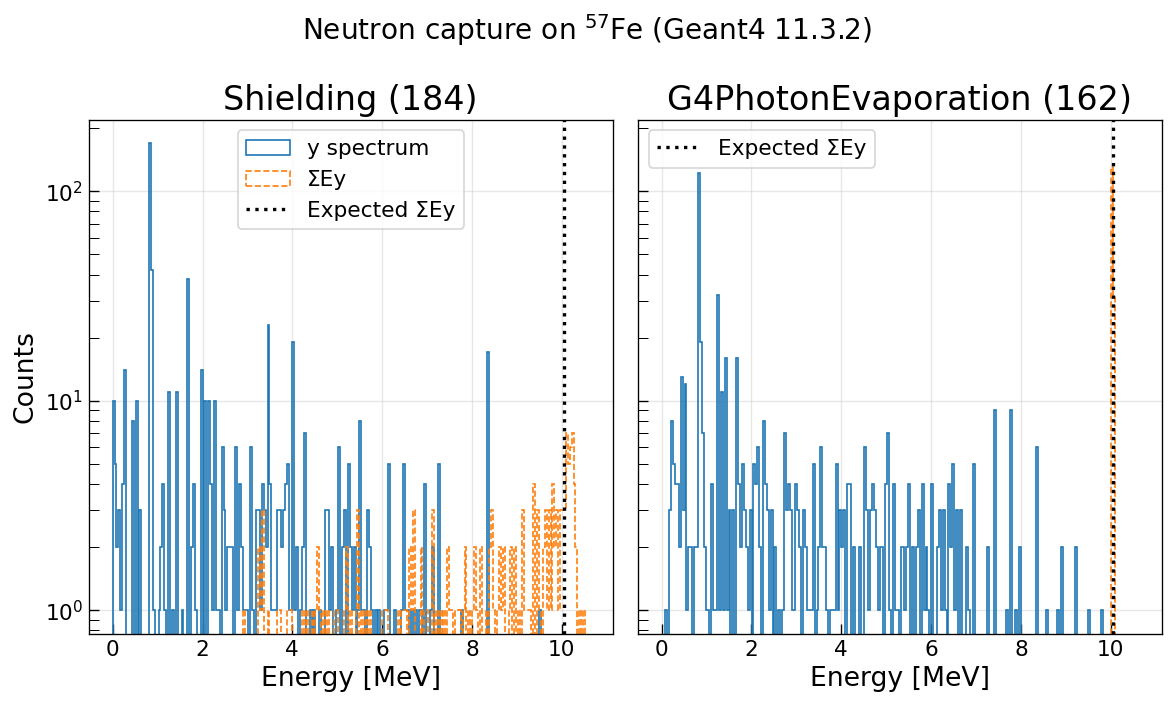
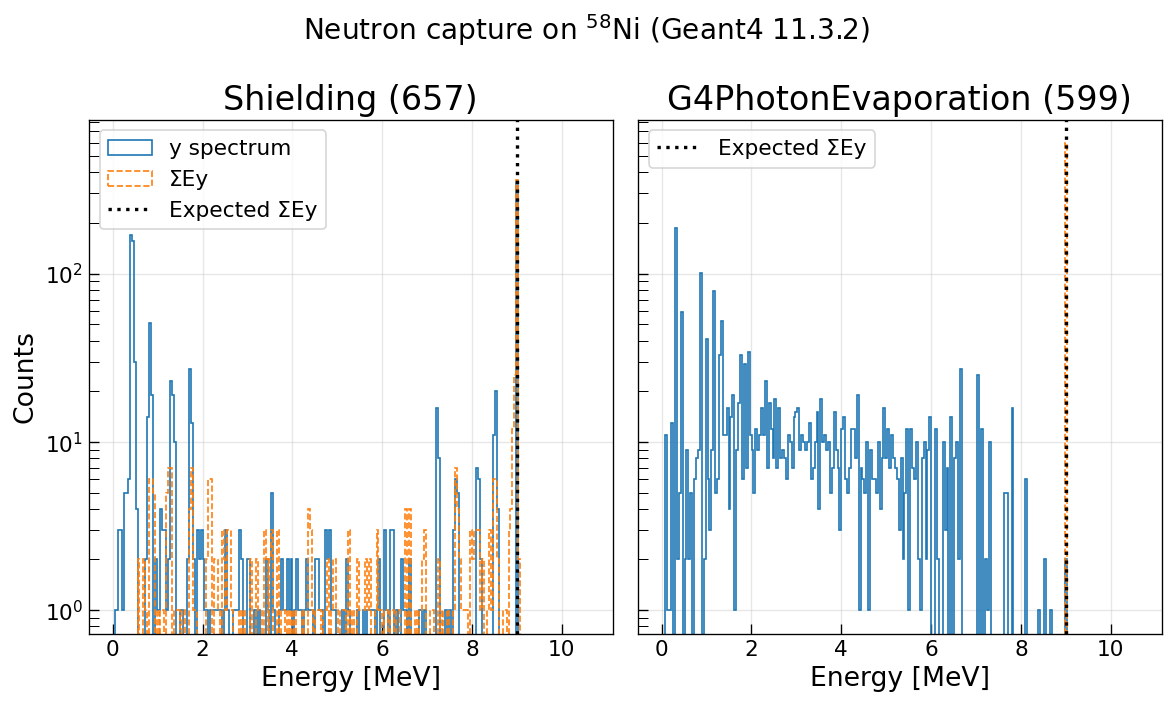
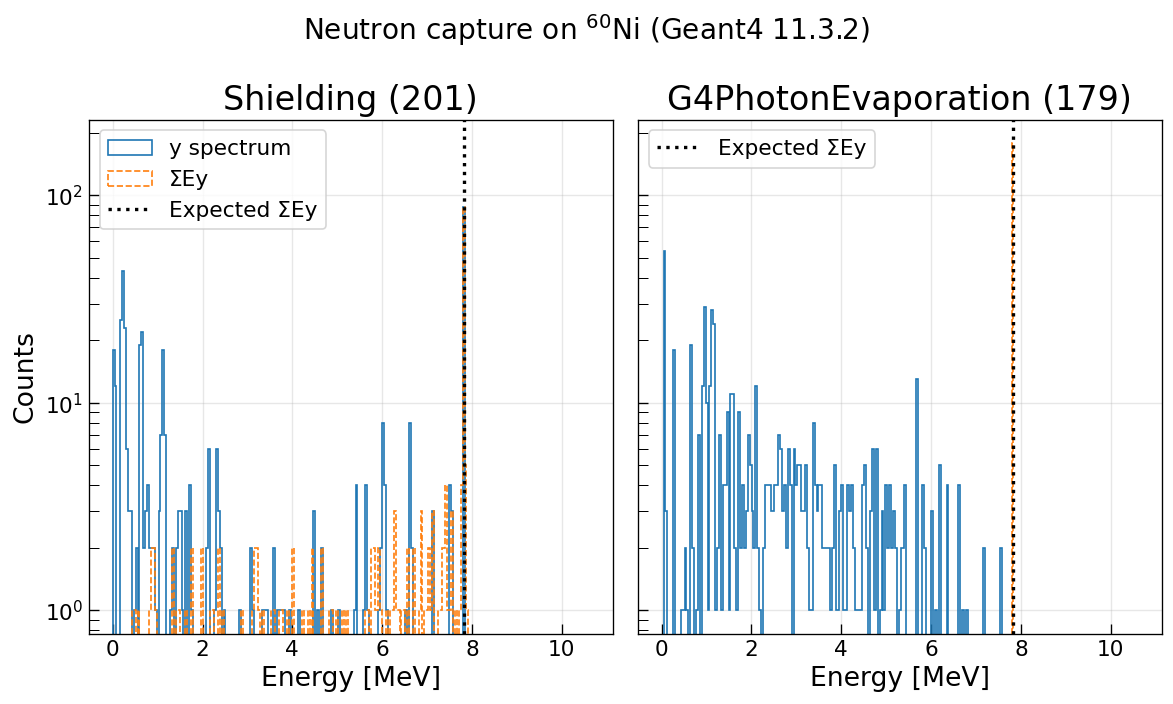
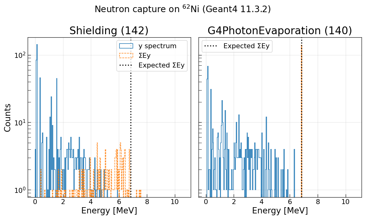
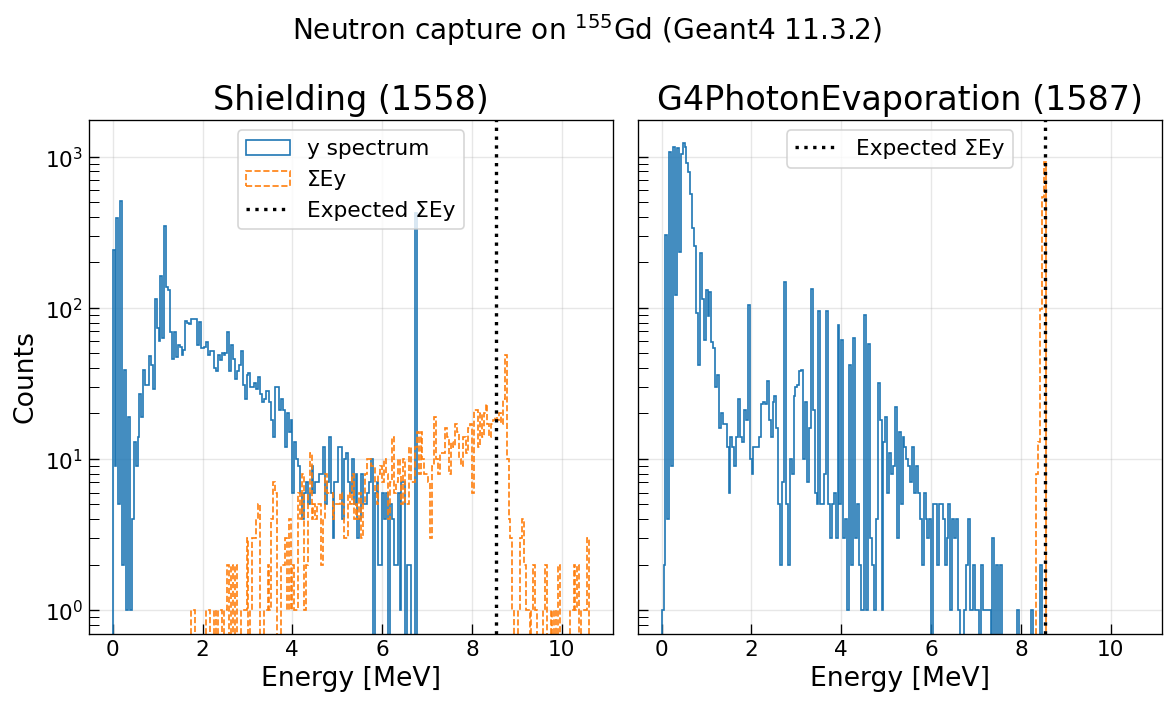
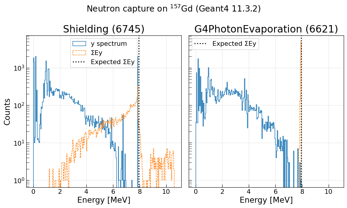
The neutron capture gamma de-excitation can be validated against literature values. Hydrogen has a well-known singular gamma line at 2.22 MeV after a neutron capture, making bugs very easy to spot. Gadolinium on the contrary, has a very complex gamma line intensity, which can be compared to publications. The Q-Values of the neutron capture process is well known for all captures in this setup. The expected Q-value according to the IAEA Nuclear Data Section is shown in each plot for the respective isotope. This can directly be compared with the orange line, depicting the summed energy of all secondary particles resulting from the neutron capture process in Geant4. In blue, the gamma line intensity is shown.

For every isotope there are always two plots shown. The plot on the left just specifies the basic G4Shielding physicslist to the simulation without any extra modifications. This means the Neutron_HP model is used, which is also used by all other relevant hadronic physiclists. As mentioned previously, this model references the gamma intensities from the G4NDL data library. The plot on the right instead additionally forces the G4PhotonEvaporation model to be used by specifying the macro command /process/had/particle_hp/use_photo_evaporation true. The G4PhotonEvaporation model should always correctly respect the Q-value of the capture, but is very likely to not correctly represent the gamma line intensity. The standard G4Shielding option might fall back to the G4PhotonEvaporation depending on the available data and version. More about the models, including the extension G4Cascade can be read here. Both plots might show a different number of captures per isotope due to the random engine getting out of sync. Still numbers should be within standard deviation of another.

Only these two models are shown due to run-time constraints. Due to the complexity of the setup, the statistics will be very lacking for these plots.

Note

The orange line is not only a sum of the gamma energies, but also includes any energy contribution from the recoil nucleus and internal conversion electrons. It includes ANY secondary produced in the Geant4 process and should correctly represent the Q-value. The plot label is just for convenience.

Note

Simulation and analysis scripts are available in tests/neutrons.

Todo

• Add a more detailed test for the cross-sections of Germanium.

• Also overlay recent experimental data from EXFOR.

• Add a simple check for C and O